38 excel bar graph labels

How to Add Percentages to Excel Bar Chart - Excel Tutorials If we would like to add percentages to our bar chart, we would need to have percentages in the table in the first place. We will create a column right to the column points in which we would divide the points of each player with the total points of all players. We will select range A1:C8 and go to Insert >> Charts >> 2-D Column >> Stacked Column ... Add or remove data labels in a chart Add data labels to a chart Click the data series or chart. To label one data point, after clicking the series, click that data point. In the upper right corner, next to the chart, click Add Chart Element > Data Labels. To change the location, click the arrow, and choose an option.

How to Change Excel Chart Data Labels to Custom Values? Go to Formula bar, press = and point to the cell where the data label for that chart data point is defined. Repeat the process for all other data labels, one after another. See the screencast. Points to note: This approach works for one data label at a time. So if you have a large chart, you are in for a lot of clicks and manic mouse maneuvering.

Excel bar graph labels

Change axis labels in a chart in Office The chart uses text from your source data for axis labels. To change the label, you can change the text in the source data. If you don't want to change the text of the source data, you can create label text just for the chart you're working on. In addition to changing the text of labels, you can also change their appearance by adjusting formats. How to rotate axis labels in chart in Excel? Rotate axis labels in chart of Excel 2013 If you are using Microsoft Excel 2013, you can rotate the axis labels with following steps: 1. Go to the chart and right click its axis labels you will rotate, and select the Format Axis from the context menu. 2. Every-other vertical axis label for my bar graph is being ... Original Title: "Bar Graphs" I am using excel 2008 for Mac and I have been trying to create a bar graph that pulls all the labels on my Vertical Category Axis, but it keeps skipping every other one. I am able to get the information graphed for each item, but the label won't come through for each item.

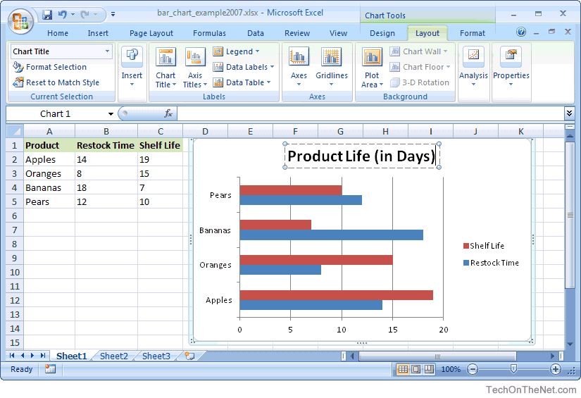
Excel bar graph labels. Text Labels on a Horizontal Bar Chart in Excel - Peltier Tech On the Excel 2007 Chart Tools > Layout tab, click Axes, then Secondary Horizontal Axis, then Show Left to Right Axis. Now the chart has four axes. We want the Rating labels at the bottom of the chart, and we'll place the numerical axis at the top before we hide it. In turn, select the left and right vertical axes. How to Use Cell Values for Excel Chart Labels Select the chart, choose the "Chart Elements" option, click the "Data Labels" arrow, and then "More Options.". Uncheck the "Value" box and check the "Value From Cells" box. Select cells C2:C6 to use for the data label range and then click the "OK" button. The values from these cells are now used for the chart data labels. Bar Chart in Excel (Examples) | How to Create Bar Chart in ... Bar Chart in Excel is one of the easiest types of the chart to prepare by just selecting the parameters and values available against them. We must have at least one value for each parameter. Bar Chart is shown horizontally, keeping their base of the bars at Y-Axis. How to Create a Bar Chart With Labels Inside Bars in Excel In a previous blog post I showed you how to put the category and data labels above the bars in a bar chart as per the graph below. Let's build this chart in Excel. Here is the dataset for the graphic in the range A5:B16—showing, as per The Guardian , the distribution of the world's top 100 footballers by country—as per the screenshot below:

How to group (two-level) axis labels in a chart in Excel? (1) In Excel 2007 and 2010, clicking the PivotTable > PivotChart in the Tables group on the Insert Tab; (2) In Excel 2013, clicking the Pivot Chart > Pivot Chart in the Charts group on the Insert tab. 2. In the opening dialog box, check the Existing worksheet option, and then select a cell in current worksheet, and click the OK button. 3. How to add total labels to stacked column chart in Excel? Add total labels to stacked column chart in Excel Supposing you have the following table data. 1. Firstly, you can create a stacked column chart by selecting the data that you want to create a chart, and clicking Insert > Column, under 2-D Column to choose the stacked column. See screenshots: And now a stacked column chart has been built. 2. Add / Move Data Labels in Charts - Excel & Google Sheets ... Change Position of Data Labels. Click on the arrow next to Data Labels to change the position of where the labels are in relation to the bar chart. Final Graph with Data Labels. After moving the data labels to the Center in this example, the graph is able to give more information about each of the X Axis Series. How do I make excel label every bar in a bar chart ... Here is what I have done: Insert->Pivot Chart Click Clustered Column Right-click on graph, select Format Axis set specify unit interval to 1 Excel now just labels every 2nd bar, even though it would easily fit (I have about 150 bars) with the given label font size.

How to Create a Bar Chart With Labels Above Bars in Excel In the chart, right-click the Series "Dummy" Data Labels and then, on the short-cut menu, click Format Data Labels. 15. In the Format Data Labels pane, under Label Options selected, set the Label Position to Inside End. 16. Next, while the labels are still selected, click on Text Options, and then click on the Textbox icon. 17. How to Add Total Data Labels to the Excel Stacked Bar Chart For stacked bar charts, Excel 2010 allows you to add data labels only to the individual components of the stacked bar chart. The basic chart function does not allow you to add a total data label that accounts for the sum of the individual components. Fortunately, creating these labels manually is a fairly simply process. Edit titles or data labels in a chart The first click selects the data labels for the whole data series, and the second click selects the individual data label. Right-click the data label, and then click Format Data Label or Format Data Labels. Click Label Options if it's not selected, and then select the Reset Label Text check box. Top of Page Excel tutorial: How to customize axis labels Here you'll see the horizontal axis labels listed on the right. Click the edit button to access the label range. It's not obvious, but you can type arbitrary labels separated with commas in this field. So I can just enter A through F. When I click OK, the chart is updated. So that's how you can use completely custom labels.

MS Excel 2007: How to Create a Bar Chart

How to place labels underneath bar chart - Microsoft Community Answer jpgpinto Replied on February 20, 2012 The names are appearing below the chart axis, that is on value 0.0%. They are on the correct place. If you want them to appear at the bottom of your chart, just select the axis and on the "Format axis" dialog box, on the "Axis options" tab, on the "Axis labels:" option, select "Low". jpgpinto

Quickly Create A Year Over Year Comparison Bar Chart In Excel

How to Make a Bar Chart in Microsoft Excel To add axis labels to your bar chart, select your chart and click the green "Chart Elements" icon (the "+" icon). Advertisement From the "Chart Elements" menu, enable the "Axis Titles" checkbox. Axis labels should appear for both the x axis (at the bottom) and the y axis (on the left). These will appear as text boxes.

Excel quartile chart - i'd like to put values over a simple bar/column

Create a multi-level category chart in Excel - ExtendOffice Select the dots, click the Chart Elements button, and then check the Data Labels box. 23. Right click the data labels and select Format Data Labels from the right-clicking menu. 24. In the Format Data Labels pane, please do as follows. 24.1) Check the Value From Cells box;

Advanced Graphs Using Excel : create line plot with error bar plot in excel

Change axis labels in a chart - support.microsoft.com Right-click the category labels you want to change, and click Select Data. In the Horizontal (Category) Axis Labels box, click Edit. In the Axis label range box, enter the labels you want to use, separated by commas. For example, type Quarter 1,Quarter 2,Quarter 3,Quarter 4. Change the format of text and numbers in labels

Bar-Line (XY) Combination Chart in Excel - Peltier Tech Blog

Change the format of data labels in a chart To get there, after adding your data labels, select the data label to format, and then click Chart Elements > Data Labels > More Options. To go to the appropriate area, click one of the four icons ( Fill & Line, Effects, Size & Properties ( Layout & Properties in Outlook or Word), or Label Options) shown here.

Resize the Plot Area in Excel Chart - Titles and Labels Overlap - YouTube

Excel charts: add title, customize chart axis, legend and ... Click anywhere within your Excel graph to activate the Chart Tools tabs on the ribbon. On the Layout tab, click Chart Title > Above Chart or Centered Overlay. Link the chart title to some cell on the worksheet For most Excel chart types, the newly created graph is inserted with the default Chart Title placeholder.

Right-aligning Y-axis labels on a stacked bar chart : excel

How to add Axis Labels (X & Y) in Excel & Google Sheets ... Excel offers several different charts and graphs to show your data. In this example, we are going to show a line graph that shows revenue for a company over a five-year period. In the below example, you can see how essential labels are because in this below graph, the user would have trouble understanding the amount of revenue over this period.

Column Graphs vs. Bar Charts – When to choose each one | Think Outside The Slide

Bar Graph in Excel — All 4 Types Explained Easily To create a simple bar graph, follow these steps: Get your Data ready. Make sure it has one categorical variable and one quantitative secondary variable. In my example from Sheet1, I have the time duration of 6 tasks. Select your Data with headers. Locate and click on the 2-D Clustered Bars option under the Charts group in the Insert Tab.

Share :