43 excel pivot table column labels
How to add column labels in pivot table [SOLVED] Re: How to add column labels in pivot table Hi BusyGurl, I have managed to do this, Excel inbuilt help has enlightened me. Steps:- Click any date in the Column Lables Click Pivot table options tab on the Ribbon. In the Options Table, Click Group Field option. Click Months then click Ok. Thats it. check the attached file:- Attached Files Pivot table row labels side by side - Excel Tutorials - OfficeTuts Excel You can copy the following table and paste it into your worksheet as Match Destination Formatting. Now, let's create a pivot table ( Insert >> Tables >> Pivot Table) and check all the values in Pivot Table Fields. Fields should look like this. Right-click inside a pivot table and choose PivotTable Options…. Check data as shown on the image below.
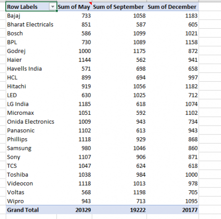
Pivot table row labels in separate columns • AuditExcel.co.za Our preference is rather that the pivot tables are shown in tabular form (all columns separated and next to each other). You can do this by changing the report format. So when you click in the Pivot Table and click on the DESIGN tab one of the options is the Report Layout. Click on this and change it to Tabular form.
Excel pivot table column labels
How To Remove Blank Row Labels In Pivot Table How to hide blanks in pivot table ms excel 2017 hide blanks in a pivot table empty field in an excel pivot table ms excel 2010 hide blanks in a pivot table Excel 2016 Pivot table Row and Column Labels - Microsoft Community In Excel 2016 I've found when I create a pivot table it unhelpfully shows 'Row Labels' and 'Column Labels' instead of my field names, although in the top left cell it says 'Count of' and then inserts the correct field name. Years ago when I last used Excel it automatically put the field names in all three heading cells. Data Labels in Excel Pivot Chart (Detailed Analysis) 7 Suitable Examples with Data Labels in Excel Pivot Chart Considering All Factors 1. Adding Data Labels in Pivot Chart 2. Set Cell Values as Data Labels 3. Showing Percentages as Data Labels 4. Changing Appearance of Pivot Chart Labels 5. Changing Background of Data Labels 6. Dynamic Pivot Chart Data Labels with Slicers 7.
Excel pivot table column labels. Excel Pivot Tables - Page 19 - by contextures.com If you have adjusted your pivot table column widths, and you want them to stay that way, you can change a setting in the pivot table options. Right-click any cell in the pivot table, and click PivotTable Options. In the PivotTable Options window, click the Format tab. In the Format section, remove the check mark from Autofit column widths on ... vba sorting pivot table columns by column field label (a date) Hi all, I have a pivot table with multiple row fields and multiple column fields. One of the column fields is a Date and I need some VBA that will auto-sort the columns into ascending order by the Date column field. E.g., if the first four column labels are "2-Jun-2010, 13-May-2009... excel - Custom column labels in PivotTable - Stack Overflow Select the data from which the pivot table is from highlight the column in which the "b" is in find and replace all the "b" with "In Progress" Update the Pivot table OR Copy the data from the pivot table and Paste it as text delimited I believe. -Change the "b" to "In Progress" Please respond if it isnt clear so I can go into further detail. How to rename group or row labels in Excel PivotTable? - ExtendOffice Click at the PivotTable, then click Analyze tab and go to the Active Field textbox. 2. Now in the Active Field textbox, the active field name is displayed, you can change it in the textbox. You can change other Row Labels name by clicking the relative fields in the PivotTable, then rename it in the Active Field textbox.
Design the layout and format of a PivotTable Change the way item labels are displayed in a layout form Change the field arrangement in a PivotTable Add fields to a PivotTable Copy fields in a PivotTable Rearrange fields in a PivotTable Remove fields from a PivotTable Change the layout of columns, rows, and subtotals Change the display of blank cells, blank lines, and errors How to Group Columns in Excel Pivot Table (2 Methods) Follow the below steps to create the expected Pivot Table. Steps: First, go to the source data sheet and press Alt + D + P from the keyboard. As a result, the PivotTable and PivotChart Wizard will show up. Click on the Multiple consolidation ranges and PivotTable options as below screenshot and press Next. Use column labels from an Excel table as the rows in a Pivot Table ... Highlight your current table, including the headers Then from the Data section of the ribbon, select From Table Highlight all the columns containing data, but not the Year column, and then select Unpivot Columns Close the dialog and keep the changes. Excel should place the unpivoted data into a new worksheet, looking something like this: Repeat item labels in a PivotTable - support.microsoft.com Right-click the row or column label you want to repeat, and click Field Settings. Click the Layout & Print tab, and check the Repeat item labels box. Make sure Show item labels in tabular form is selected. Notes: When you edit any of the repeated labels, the changes you make are applied to all other cells with the same label.
Centre Column Headings in Excel Pivot Table To centre the column headings in Excel 2007: Select a cell in the pivot table. On the Ribbon, under the PivotTable Tools tab, click Options. At the far left, in the PivotTable group, click Options. On the Layout & Format tab, in the Layout section, add a check mark to Merge and Center Cells With Labels. Click OK. Automatic Row And Column Pivot Table Labels - How To Excel At Excel Select the data set you want to use for your table The first thing to do is put your cursor somewhere in your data list Select the Insert Tab Hit Pivot Table icon Next select Pivot Table option Select a table or range option Select to put your Table on a New Worksheet or on the current one, for this tutorial select the first option Click Ok Pivot Table column label from horizontal to vertical After pivot table and with grouping, some column labels have been showed but the caption is on the top. What i want is put the column header at the left of the row as vertical red text show as below. However, i cannot do this, it said "We cant change this part of pivot table". What can i do for this case if necessary? I have attached the file FYR. How To Add Two Columns Values In Pivot Table Excel Add multiple columns to a pivot table custuide add multiple columns to a pivot table custuide ms excel 2010 display the fields in values section multiple columns a pivot table how to make row labels on same line in pivot table. Share this: Click to share on Twitter (Opens in new window)
How to Make a Pivot Table in Excel versions: 365, 2019, 2016 and 2013 [Includes Pivot Chart]
How to Use Excel Pivot Table Label Filters - Contextures Excel Tips Right-click on an item in the Row Labels or Column Labels In the pop-up menu, click Filter, then click Hide Selected Items. The item is immediately hidden in the pivot table. Quickly Hide All But a Few Items You can use a similar technique to hide most of the items in the Row Labels or Column Labels.

Excel Pivot Table Report - Sort Data in Row & Column Labels & in Values Area, use Custom Lists
How to make row labels on same line in pivot table? - ExtendOffice As we all know, the pivot table has several layout form, the tabular form may help us to put the row labels next to each other. Please do as follows: 1. Click any cell in your pivot table, and the PivotTable Tools tab will be displayed. 2. Under the PivotTable Tools tab, click Design > Report Layout > Show in Tabular Form, see screenshot: 3.
Create a Pivot Table in Excel - The Complete Beginners Guide - QuickExcel
Excel Pivot Table Chart Select Data Free Table Bar Chart Go summary region using click the 4 to put months- the step drag step now to report we pivot table have and I sum together wise excel- heading summary pivot a t. Otosection Home; News; Technology. All; Coding; Hosting; Create Device Mockups in Browser with DeviceMock.

Pivot Table Tip- Assign The Correct Row And Column Labels Quickly - How To Excel At Excel
Data Labels in Excel Pivot Chart (Detailed Analysis) 7 Suitable Examples with Data Labels in Excel Pivot Chart Considering All Factors 1. Adding Data Labels in Pivot Chart 2. Set Cell Values as Data Labels 3. Showing Percentages as Data Labels 4. Changing Appearance of Pivot Chart Labels 5. Changing Background of Data Labels 6. Dynamic Pivot Chart Data Labels with Slicers 7.

excel - VBA - How do I group columns in a pivot table, collapse the group, and rename the label ...
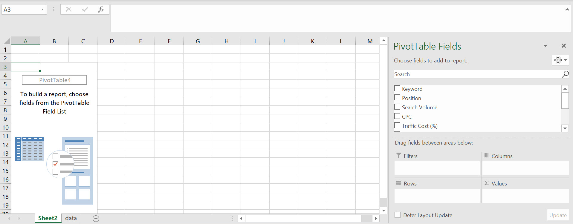
Excel 2016 Pivot table Row and Column Labels - Microsoft Community In Excel 2016 I've found when I create a pivot table it unhelpfully shows 'Row Labels' and 'Column Labels' instead of my field names, although in the top left cell it says 'Count of' and then inserts the correct field name. Years ago when I last used Excel it automatically put the field names in all three heading cells.
How-to Make an Excel Stacked Column Pivot Chart with a Secondary Axis - Excel Dashboard Templates
How To Remove Blank Row Labels In Pivot Table How to hide blanks in pivot table ms excel 2017 hide blanks in a pivot table empty field in an excel pivot table ms excel 2010 hide blanks in a pivot table

MVP #10: Making a Pivot table that has labels spread across several columns | Productivity Tips ...

Can I use the union of two columns values in Excel as row labels in a Pivot Table? - Super User
microsoft excel - Grouping labels and concatenating their text values (like a pivot table ...

How to Insert an Excel Pivot Table - YouTube

Excel Help: Simple method to make Pivot table
MS Excel pivot table - expand column in a new sheet - Stack Overflow
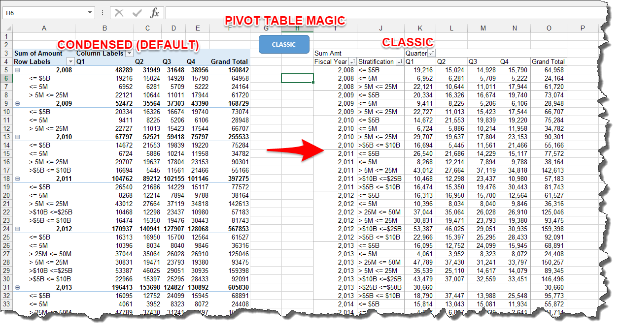
Microsoft Excel — Pivot Table Magic - Let’s Excel - Medium

Design your Pivot Table in Excel | Excel in Excel

23 things you should know about Excel pivot tables | Exceljet

How to Sort Data in a Pivot Table | Excelchat

Pivot Table in Microsoft Excel - Pivot Table Field List Report Functions of Filter Column Labels ...
Post a Comment for "43 excel pivot table column labels"